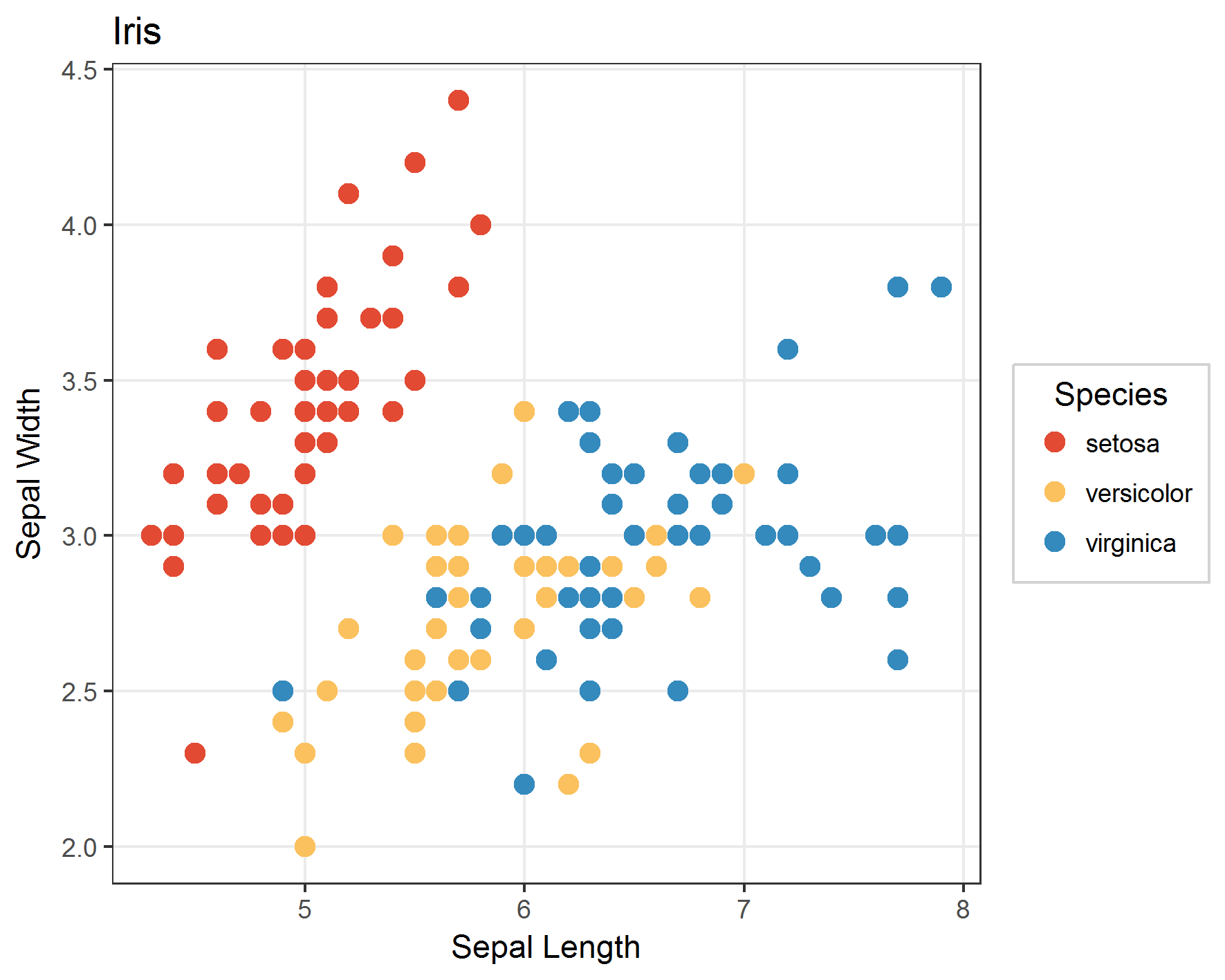
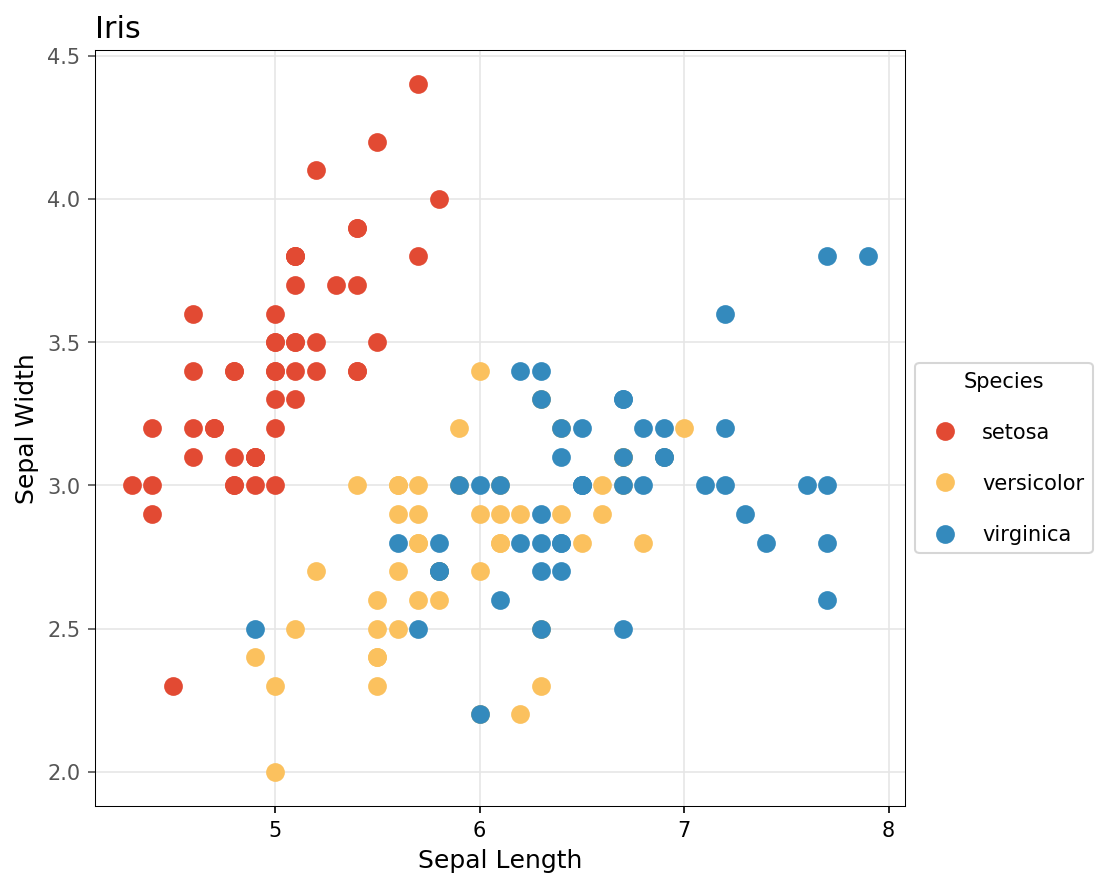
This is a fun post, where I wanted to try to make a matplotlib figure similar to a ggplot figure. Can you guess which image was created with matplotlib and which with ggplot? The answer can be found here.
To make the matplotlib similar to the ggplot you can pass on a style argument. There is a ggplot style already available but I personally prefer the white background as in ggplot’s theme_bw. So I adapted the mplstyle file and put it on Gist.
If you want to use this style download the file and specify in Python the path to this file, e.g.
import matplotlib.pyplot as plt
theme_bw = "path2file/theme_bw.mplstyle"
plt.style.use(theme_bw)
You can also put the theme_bw.mplstyle into your matplotlib folder (Python -> Lib -> site-packages -> matplotlib -> mpl-data -> stylelib), then you can load the style more easily with
plt.style.use("theme_bw")Here is the full code to generate the two figures above. I had to make a few tweaks to make them as similar as possible.
In R with ggplot:
library(ggplot2)
# Define colors
cols <- c("setosa" = "#E24A33", "virginica" = "#348ABD", "versicolor" = "#FBC15E")
g <- ggplot(data = iris, aes(x = Sepal.Length, y = Sepal.Width, col = factor(Species))) +
  geom_point(size = 3) +
  theme_bw() +
  xlab("Sepal Length") +
  ylab("Sepal Width") +
  ggtitle("Iris") +
  scale_colour_manual(values = cols) +
  guides(col = guide_legend(title = "Species")) +
  theme(legend.title.align = 0.5,
    legend.background = element_rect(colour = 'lightgrey', linetype = 'solid'))
g
And in Python with matplotlib:
import pandas as pd
import matplotlib.pyplot as plt
import numpy as np
from sklearn import datasets
# Load the theme_bw matplotlib theme
theme_bw = "path2file/theme_bw.mplstyle"
plt.style.use(theme_bw)
# Load the famous iris data
iris = datasets.load_iris()
# Convert to pandas data frame and rename columns
df = pd.DataFrame(data = np.c_[iris['data'], iris['target']],
                     columns = iris['feature_names'] + ['target'])
df.rename(columns = {'sepal length (cm)': 'sepal_length',
                     'sepal width (cm)': 'sepal_width',
                     "petal length (cm)": "petal_length",
                     "petal width (cm)": "petal_width",
                     "target": "species"}, inplace=True)
# Specify colors
col = ["#E24A33", "#FBC15E", "#348ABD"]
species = ["setosa", "versicolor", "virginica"]
# Plot
fig = plt.figure(figsize = (9, 7.2), dpi = 50)
ax = plt.subplot(111)
# A few tweaks to save the image in the same aspect ratio as the R graphic
fig.subplots_adjust(top = 0.8,
                    bottom = 0.1,
                    left = 0.1,
                    right = 0.9)
# Add plot for each species
for i in np.unique(df["species"]):
    ax.plot(df[df["species"] == i]["sepal_length"],
            df[df["species"] == i]["sepal_width"], "o", markersize = 8,
            c = col[int(i)], label = species[int(i)])
plt.ylabel("Sepal Width")
plt.xlabel("Sepal Length")
plt.title("Iris", loc = "left")
# Add space for legend on the right
box = ax.get_position()
ax.set_position([box.x0, box.y0, box.width * 0.75, box.height])
# Add legend
ax.legend(bbox_to_anchor = (1, 0.6), title = "Species", labelspacing = 1.5)
# Remove minor ticks on x axis
plt.xticks(np.arange(5, max(df.sepal_length) + 1, 1.0))
plt.show()
To answer the initial question: The left plot above has been created with ggplot in R, the right plot with matplotlib in Python.